T-GCN: A Temporal Graph ConvolutionalNetwork for Traffic Prediction (1811.05320v3)

Abstract: Accurate and real-time traffic forecasting plays an important role in the Intelligent Traffic System and is of great significance for urban traffic planning, traffic management, and traffic control. However, traffic forecasting has always been considered an open scientific issue, owing to the constraints of urban road network topological structure and the law of dynamic change with time, namely, spatial dependence and temporal dependence. To capture the spatial and temporal dependence simultaneously, we propose a novel neural network-based traffic forecasting method, the temporal graph convolutional network (T-GCN) model, which is in combination with the graph convolutional network (GCN) and gated recurrent unit (GRU). Specifically, the GCN is used to learn complex topological structures to capture spatial dependence and the gated recurrent unit is used to learn dynamic changes of traffic data to capture temporal dependence. Then, the T-GCN model is employed to traffic forecasting based on the urban road network. Experiments demonstrate that our T-GCN model can obtain the spatio-temporal correlation from traffic data and the predictions outperform state-of-art baselines on real-world traffic datasets. Our tensorflow implementation of the T-GCN is available at https://github.com/lehaifeng/T-GCN.

• The paper presents the T-GCN model that integrates a GCN for spatial feature extraction and a GRU for capturing temporal dependencies in traffic data.
• It addresses complex traffic prediction challenges by modeling road network topology and dynamic traffic patterns simultaneously.
• Experimental results demonstrate that T-GCN outperforms traditional methods with lower RMSE and higher accuracy across various prediction horizons.

T-GCN: A Temporal Graph Convolutional Network for Traffic Prediction

The paper presents a novel approach for traffic prediction by introducing the Temporal Graph Convolutional Network (T-GCN). This model combines spatial and temporal dependencies of traffic data using Graph Convolutional Networks (GCN) and Gated Recurrent Units (GRU), respectively. This essay provides a detailed analysis of the methodology, results, and implications for real-world traffic forecasting.

Problem Definition and Methodology

Traffic Prediction Challenges

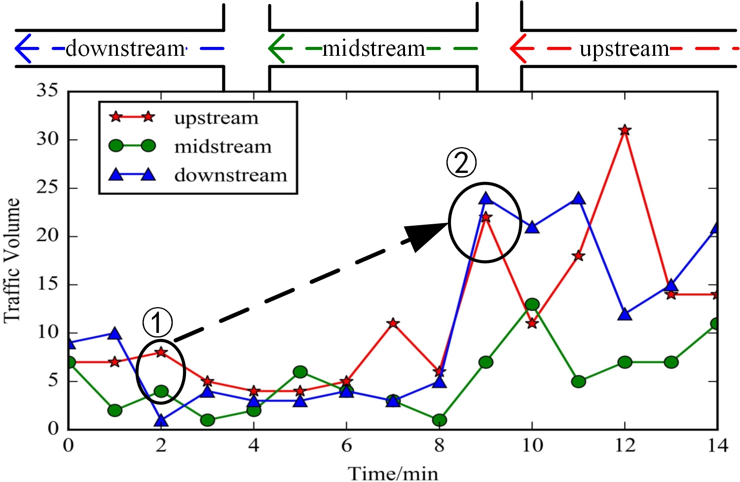
Traffic prediction involves accurately analyzing and forecasting trends in traffic conditions, which is crucial for intelligent traffic systems, urban planning, and management. This task is complicated by:

• Spatial Dependence: Traffic conditions on adjacent road networks affect each other, creating complex spatial dependencies (Figure 1).

  Figure 1: Spatial dependence is restricted by the topological structure of the road network. Due to the strong influence between adjacent roads, the short-term traffic flow similarity is changed from state \textcircled{1} to state \textcircled{2}.

• Temporal Dependence: Traffic volumes show periodic and trend-based changes over time (Figure 2).

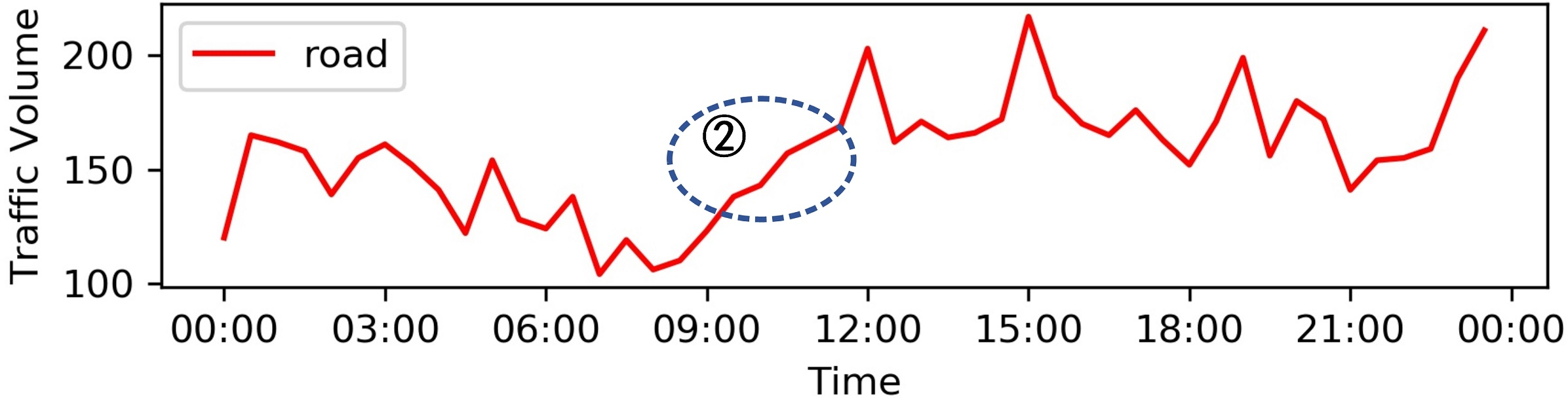
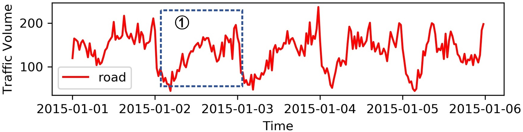
Figure 2: (a) Periodicity. The traffic volume in the road changes periodically within one week. (b) Trend. The traffic volume in the road has tendency change within one day.

Traditional methods like ARIMA and SVR fail to effectively capture the complexities of these dependencies, particularly under non-Euclidean road network structures.

T-GCN Model Architecture

The T-GCN model integrates a GCN to capture spatial dependencies and a GRU to handle temporal sequences. The GCN processes the topological network of roads, encoding the spatial structure, while the GRU captures dynamic temporal patterns through iterative data processing (Figure 3 and Figure 4).

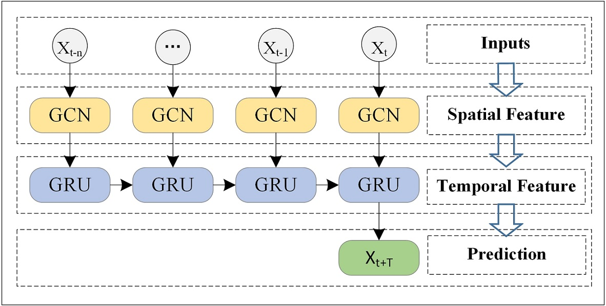
Figure 3: Overview. We take the historical traffic information as input and obtain the finally prediction result through the Graph Convolution Network and the Gated Recurrent Units model.

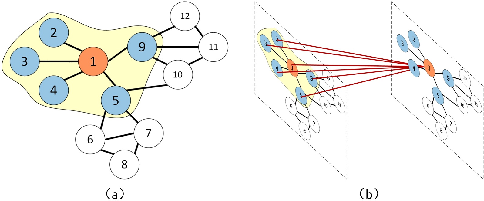
Figure 4: Assuming that node 1 is a central road. (a) The blue nodes indicate the roads connected to the central road. (b) We obtain the spatial feature by obtaining the topological relationship between the road 1 and the surrounding roads.

The temporal component uses a GRU because of its efficient structure, which, unlike LSTM, needs fewer parameters and hence speeds up the training process (Figure 5).

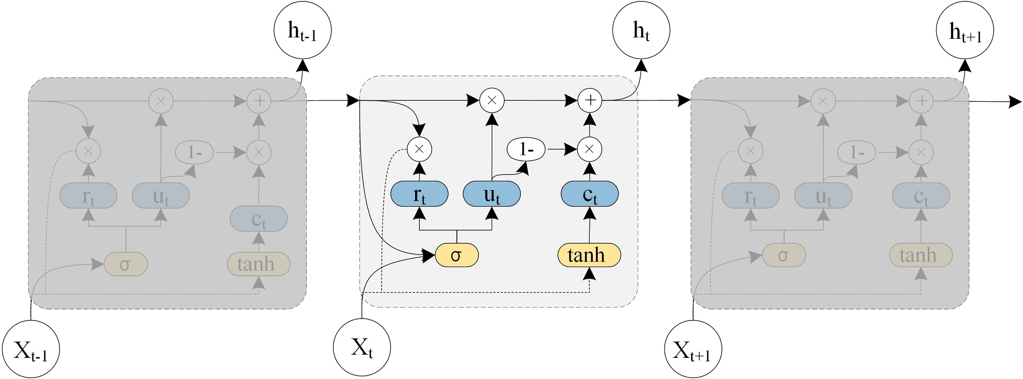
Figure 5: The architecture of the Gated Recurrent Unit model.

The combined T-GCN architecture allows simultaneous learning from both spatial and temporal features (Figure 6).

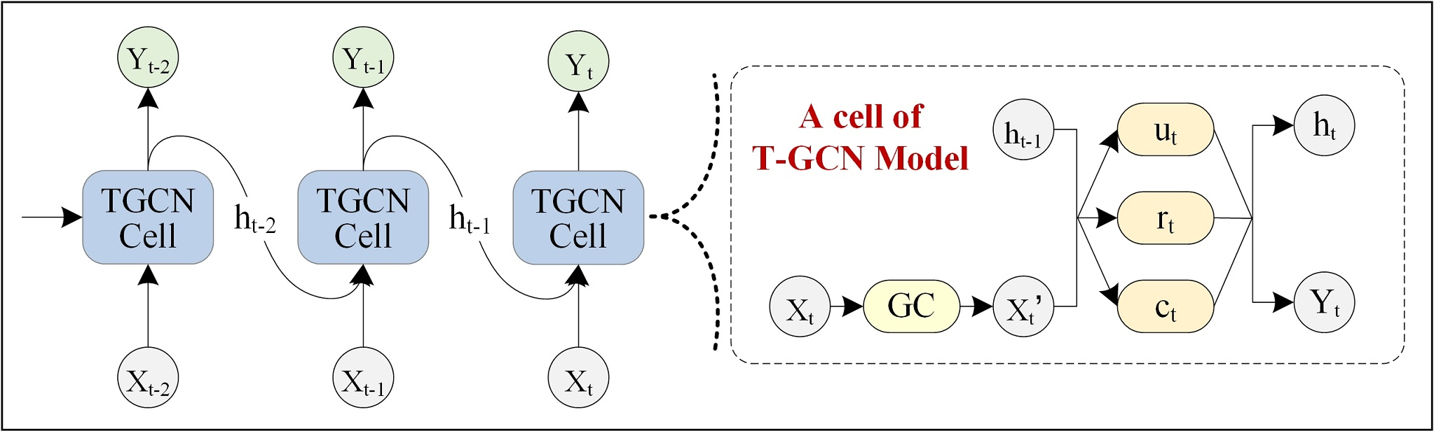
Figure 6: The overall process of spatio-temporal prediction. The right part represents the specific architecture of a T-GCN unit, and GC represents graph convolution.

Experimental Results and Analysis

Evaluation Metrics and Performance

The T-GCN model was evaluated using Root Mean Squared Error (RMSE), Mean Absolute Error (MAE), Accuracy, Coefficient of Determination ($R^2$), and Explained Variance Score. The results on real-world datasets SZ-taxi and Los-loop showed significant improvements over baseline methods (Figure 7 and Figure 8).

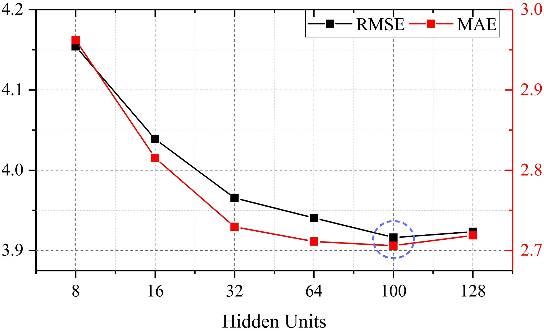
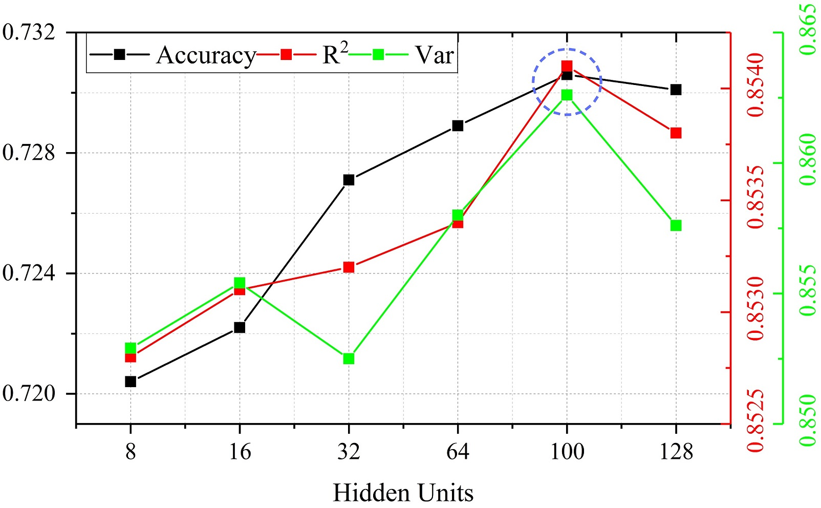
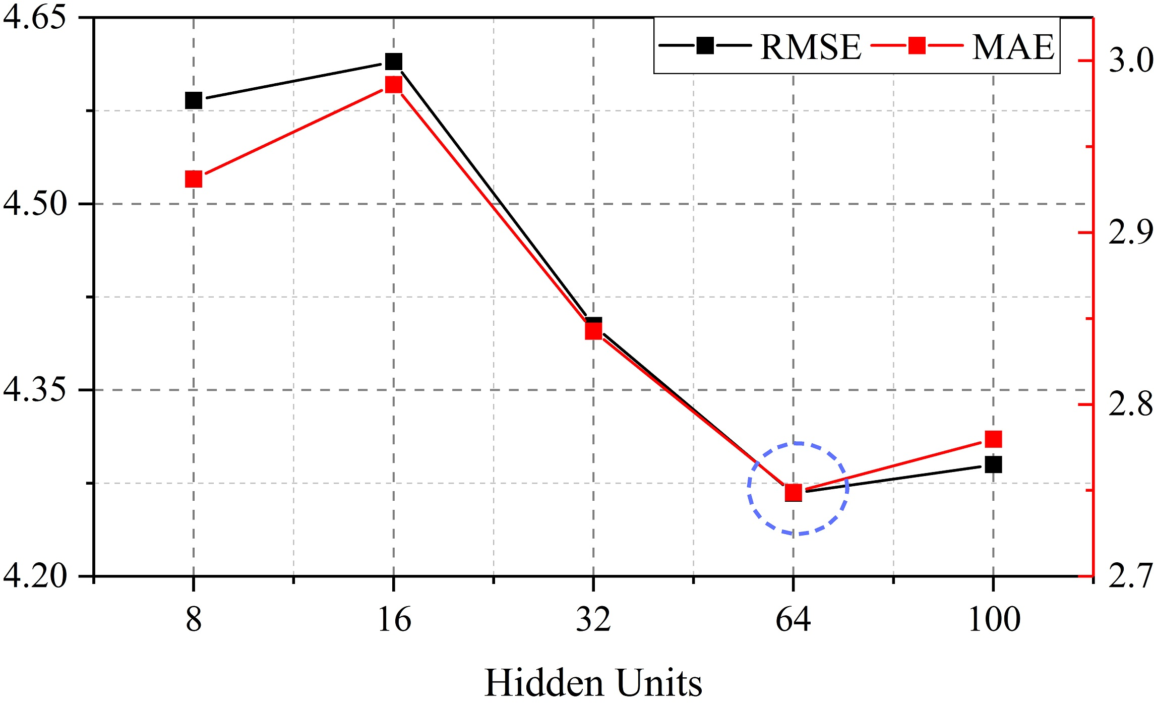
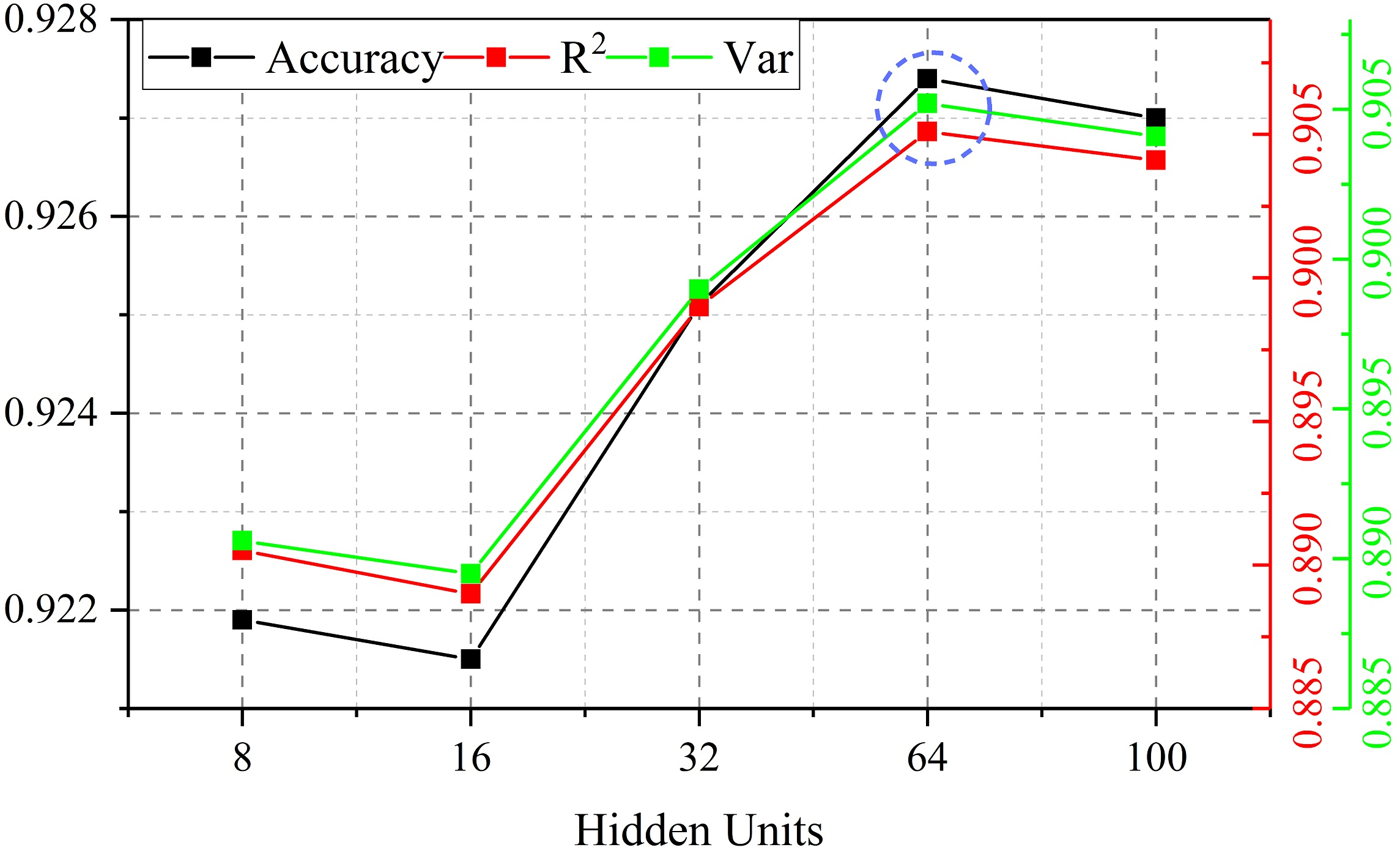
Figure 7: Comparison of predicted performance under different hidden units. (a) Changes in RMSE and MAE based on SZ-taxi. (b) Changes in Accuracy, $R^{2}$ and Var based on SZ-taxi.

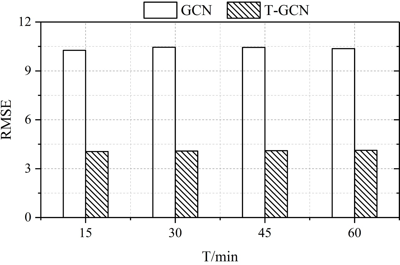
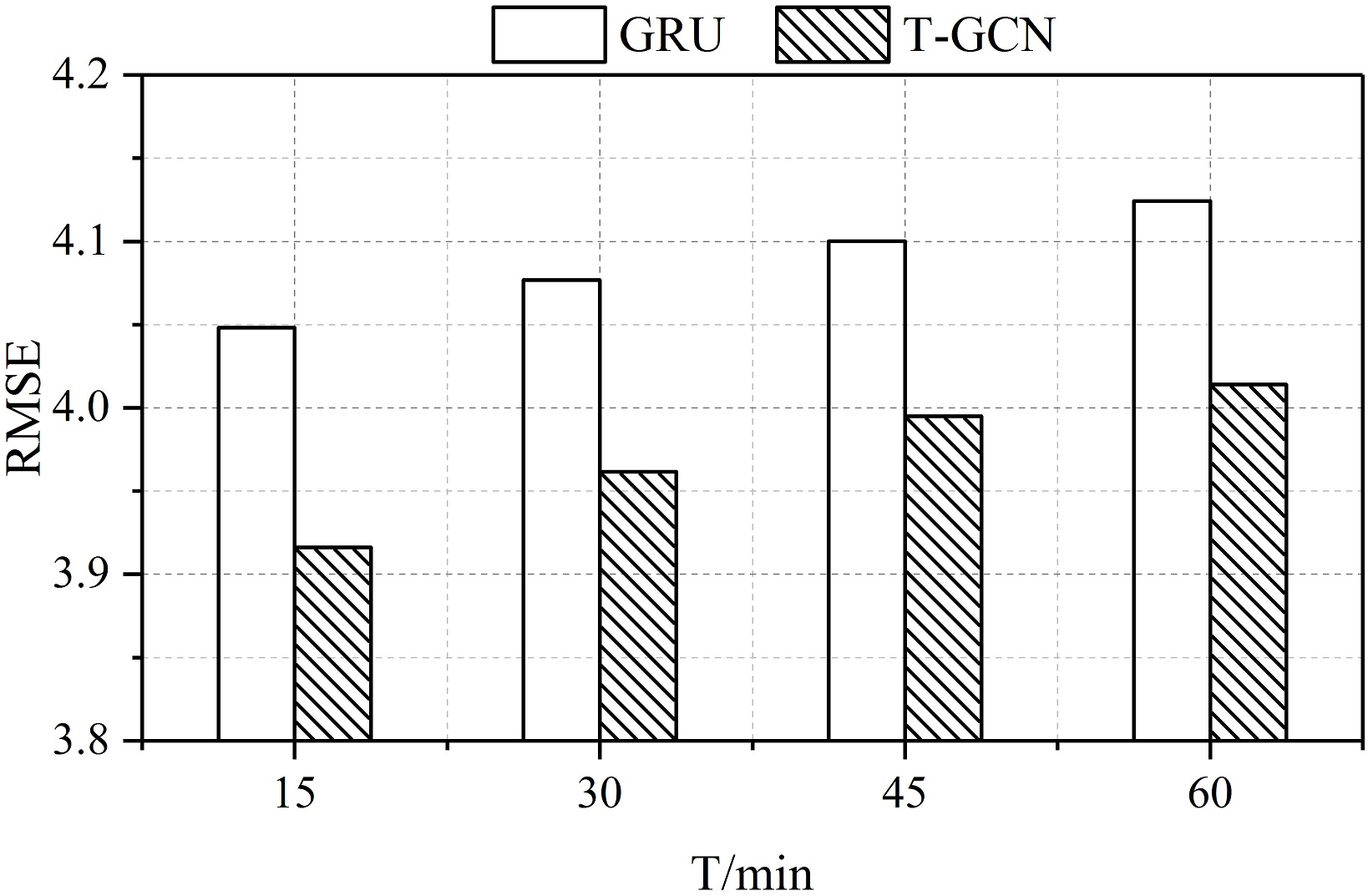
Figure 8: (a) The RMSE of the T-GCN model lower than the GCN model, which considers spatial feature only, indicating the effectiveness of the T-GCN to capture spatial feature. (b) The RMSE of the T-GCN model lower than the GRU model, which considers temporal feature only, indicating the effectiveness of the T-GCN to capture temporal feature.

Robustness and Long-term Prediction

T-GCN demonstrates robustness to noise perturbations (Figure 9) and provides consistent performance across varying prediction horizons, indicating its suitability for both short-term and long-term predictions (Figure 10).

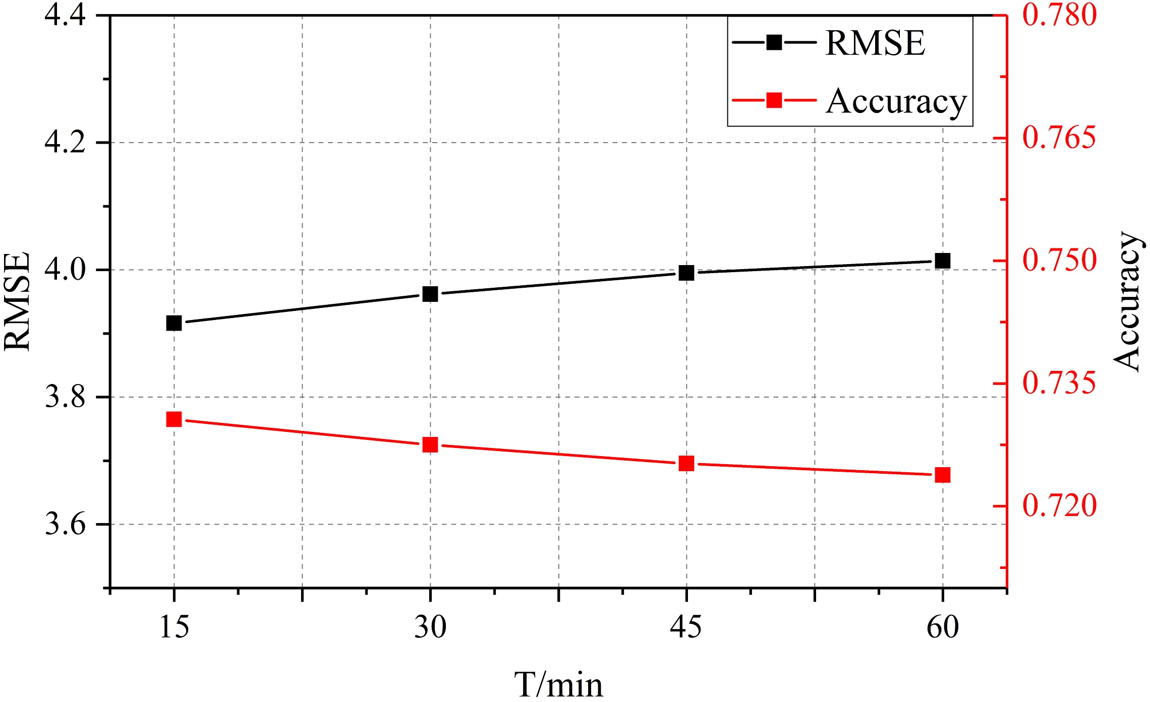
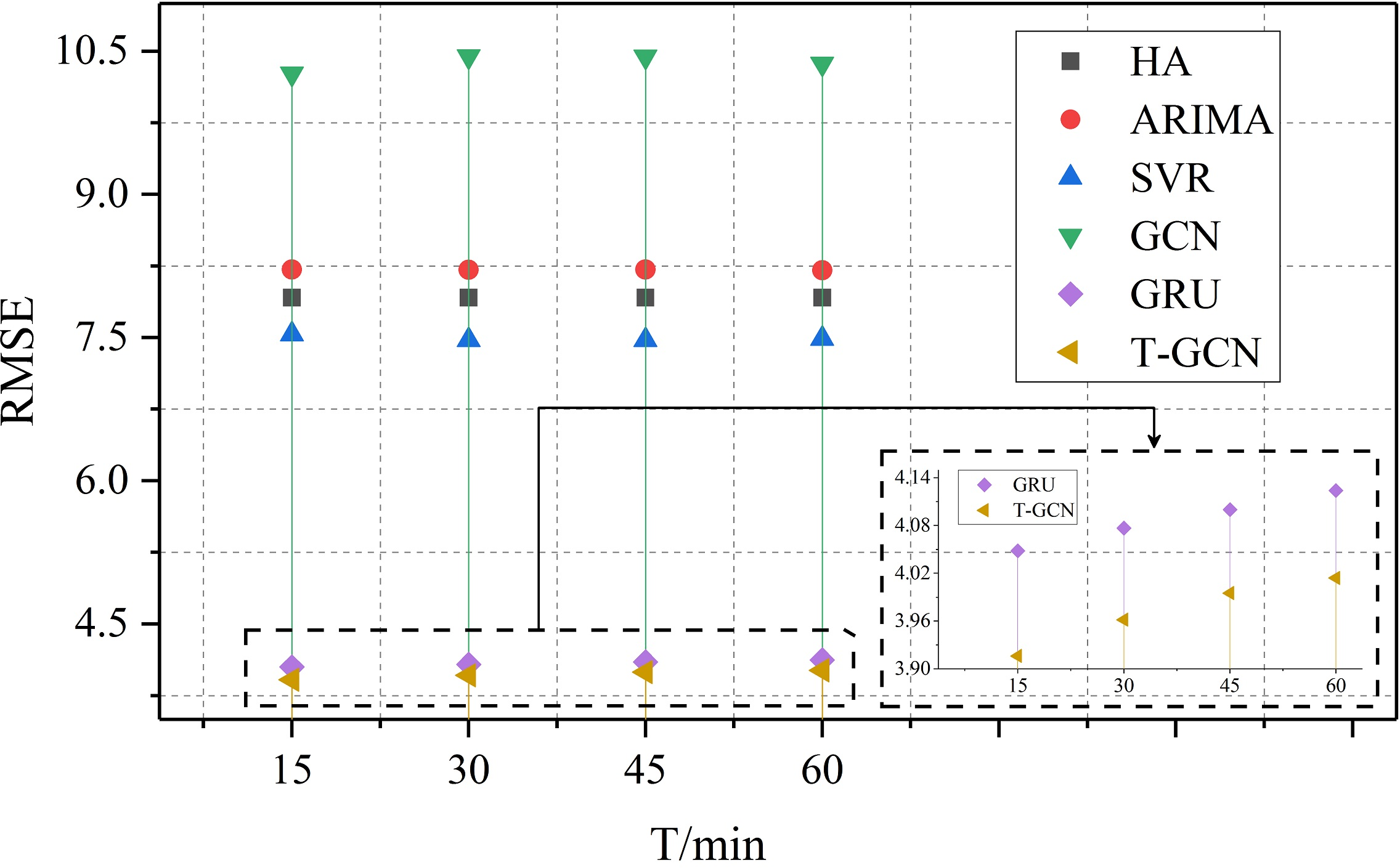
Figure 10: (a) Under different prediction horizons, the change of RMSE and Accuracy are small, indicating that our approach is insensitive to prediction horizons. (b) Under different prediction horizons, the T-GCN model has lowest RMSE error compared to baseline methods.

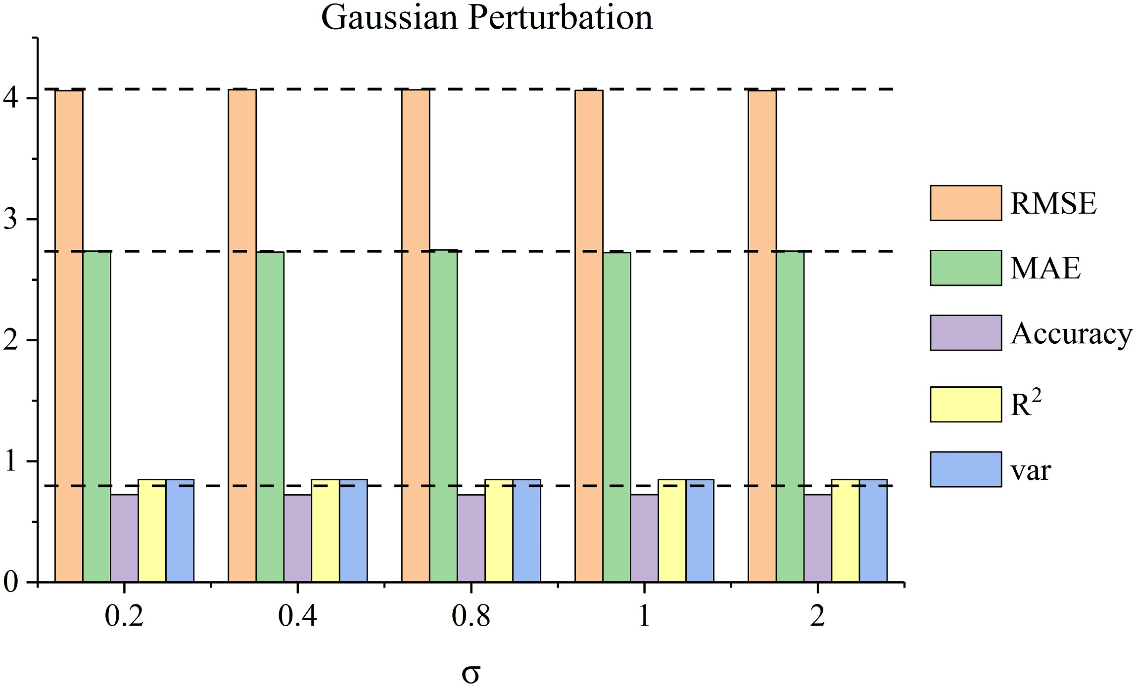
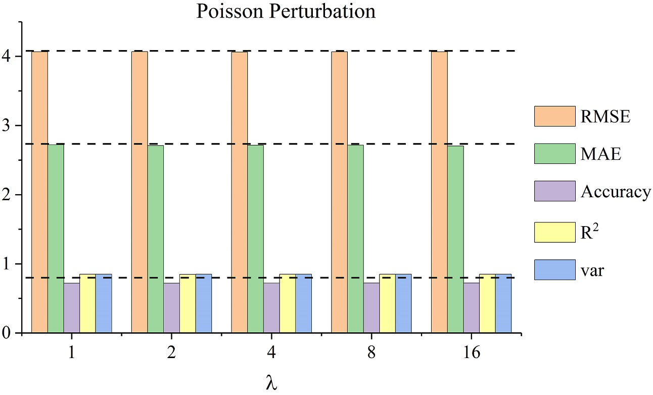
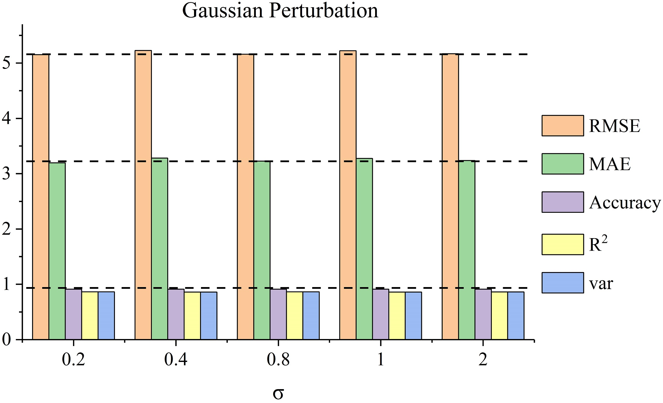
Figure 9: Perturbation analysis. The horizontal axis represents sigma or lambda, the vertical axis represents prediction results, and different colors mean different metrics. (a) The results of adding Gaussian perturbation on SZ-taxi. (b) The results of adding Poisson perturbation on SZ-taxi. (c) The results of adding Gaussian perturbation on Los-loop. (d) The results of adding Poisson perturbation on Los-loop.

Implications and Future Work

The T-GCN model harnesses the power of GCN and GRU to address the complexities in traffic prediction, demonstrating superior accuracy and robustness over traditional methods. This capability extends beyond traffic forecasting, offering potential applications in other spatio-temporal prediction tasks such as environmental monitoring and urban mobility analysis.

Future work may involve optimizing computational efficiency for larger datasets, integrating external factors such as weather conditions, and extending the model to other domains to enhance applicability and performance.

Conclusion

This paper introduces the T-GCN model as a robust solution for traffic prediction, effectively integrating spatial and temporal dependencies. It outperforms existing models and paves the way for further advancements in the domain of spatio-temporal forecasting.