A Neural Stochastic Volatility Model (1712.00504v2)

Abstract: In this paper, we show that the recent integration of statistical models with deep recurrent neural networks provides a new way of formulating volatility (the degree of variation of time series) models that have been widely used in time series analysis and prediction in finance. The model comprises a pair of complementary stochastic recurrent neural networks: the generative network models the joint distribution of the stochastic volatility process; the inference network approximates the conditional distribution of the latent variables given the observables. Our focus here is on the formulation of temporal dynamics of volatility over time under a stochastic recurrent neural network framework. Experiments on real-world stock price datasets demonstrate that the proposed model generates a better volatility estimation and prediction that outperforms mainstream methods, e.g., deterministic models such as GARCH and its variants, and stochastic models namely the MCMC-based model \emph{stochvol} as well as the Gaussian process volatility model \emph{GPVol}, on average negative log-likelihood.

• The paper introduces NSVM, which integrates deep recurrent networks with variational inference to enhance volatility estimation.
• It employs a dual network architecture, using generative and inference networks to capture complex temporal dependencies and multivariate interactions.
• Experimental results on stock datasets show that NSVM outperforms traditional GARCH and MCMC-based models in negative log-likelihood performance.

A Neural Stochastic Volatility Model

This essay discusses a paper that introduces a neural stochastic volatility model (NSVM) for estimating and predicting volatility in financial time series. The paper leverages the integration of statistical models with deep recurrent neural networks to formulate volatility models, addressing the limitations of traditional methods like GARCH and MCMC-based models. The core innovation lies in a pair of complementary stochastic recurrent neural networks: a generative network modeling the joint distribution of the stochastic volatility process and an inference network approximating the conditional distribution of latent variables.

Background and Motivation

Volatility modeling is crucial for risk management, investment decisions, and derivative pricing in finance. Traditional approaches, such as ARCH and GARCH models, rely on handcrafted features and strong assumptions about the underlying time series. While these models have been widely used, they may not capture the complex, nonlinear dynamics of volatility. Stochastic volatility (SV) models offer an alternative by specifying the variance as a latent stochastic process. However, these models often require computationally expensive sampling routines and struggle with multivariate time series.

The paper addresses these limitations by proposing a fully data-driven approach that leverages the power of recurrent neural networks (RNNs) and variational inference. By combining stochastic models with RNNs, the NSVM aims to provide a more flexible and accurate framework for volatility modeling, capable of capturing complex temporal dependencies and handling multivariate data.

Model Formulation

The NSVM builds upon the foundation of SV models but extends them with autoregressive and bidirectional architectures. The model assumes that latent variables follow a Gaussian autoregressive process, which is then used to model the variance process. The NSVM comprises two main components: a generative network and an inference network.

Generative Network

The generative network models the joint distribution of the observable sequence $X$ and the latent stochastic process $Z$. It consists of two pairs of RNNs and multi-layer perceptrons (MLPs): $\RNN^z_G$/$\MLP^z_G$ for the latent variable $Z$ and $\RNN^x_G$/$\MLP^x_G$ for the observable variable $X$. The RNNs capture the temporal dependencies in the data, while the MLPs map the hidden states of the RNNs to the means and variances of the variables of interest. The generative network is defined as follows:

$\begin{aligned} \{\mu^z_t, \Sigma^z_t\} &= \MLP^z_G(h^z_t; \ps{\Phi}), \ h^z_t &= \RNN^z_G(h^z_{t-1}, z_{t-1}; \ps{\Phi}), \ z_t &\sim \mathscr{N}(\mu^z_t, \Sigma^z_t), \ \{\mu^x_t, \Sigma^x_t\} &= \MLP^x_G(h^x_t; \ps{\Phi}), \ h^x_t &= \RNN^x_G(h^x_{t-1}, x_{t-1}, z_t; \ps{\Phi}), \ x_t &\sim \mathscr{N}(\mu^x_t, \Sigma^x_t), \end{aligned}$

where $h^z_t$ and $h^x_t$ denote the hidden states of the corresponding RNNs, and $\ps{\Phi}$ represents the collection of parameters of the generative model.

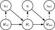
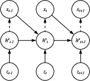
Figure 1: Two components of the generative network.

Inference Network

The inference network approximates the conditional distribution of the latent variables given the observables, $q_{\ps{\Psi}(Z | X)}$. It employs a cascaded architecture with an autoregressive RNN and a bidirectional RNN. The bidirectional RNN captures both forward and backward dependencies on the entire observation sequence, while the autoregressive RNN models the temporal dependencies on the latent variables. The inference network is defined as:

$\begin{aligned} \{\tilde{\mu}^z_t, \tilde{\Sigma}^z_t\} &= \MLP^z_I(\tilde{h}^z_{t}; \ps{\Psi}), \ \tilde{h}^z_{t} &= \RNN^z_I(\tilde{h}^z_{t-1}, z_{t-1}, [\tilde{h}^{\rightarrow}_t, \tilde{h}^{\leftarrow}_t]; \ps{\Psi}), \ \tilde{h}^{\rightarrow}_t &= \RNN^{\rightarrow}_I(\tilde{h}^{\rightarrow}_{t-1}, x_t; \ps{\Psi}), \ \tilde{h}^{\leftarrow}_t &= \RNN^{\leftarrow}_I(\tilde{h}^{\leftarrow}_{t+1}, x_t; \ps{\Psi}), \ z_t &\sim \mathscr{N}(\tilde{\mu}^z_t, \tilde{\Sigma}^z_t; \ps{\Psi}), \end{aligned}$

where $\tilde{h}^{\rightarrow}_t$ and $\tilde{h}^{\leftarrow}_t$ represent the hidden states of the forward and backward directions of the bidirectional RNN, and $\ps{\Psi}$ denotes the collection of parameters of the inference model.

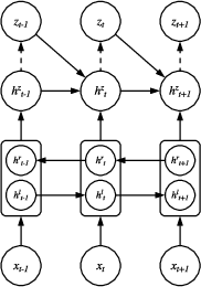
Figure 2: Architecture of the inference network.

Training and Forecasting

The model parameters are learned via variational inference, maximizing the evidence lower bound (ELBO) of the marginal log-likelihood of the observable variables. The ELBO is estimated using Monte Carlo integration with reparameterization to enable gradient-based optimization. For forecasting, the authors employ a recursive 1-step-ahead forecasting routine, where the model is updated as new observations become available.

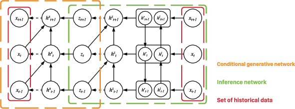
Figure 3: Illustration of the training setup.

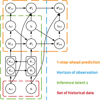
Figure 4: Illustration of the forecasting setup.

Experimental Results

The paper evaluates the NSVM on real-world stock price datasets, comparing its performance against various deterministic and stochastic volatility models, including GARCH variants, MCMC-based stochvol, and Gaussian process volatility model GP-Vol. The results demonstrate that the NSVM achieves higher accuracy in volatility estimation and prediction, as measured by negative log-likelihood (NLL). Specifically, the NSVM with rank-1 perturbation outperforms all other models, while the NSVM with a diagonal covariance matrix also shows competitive performance.

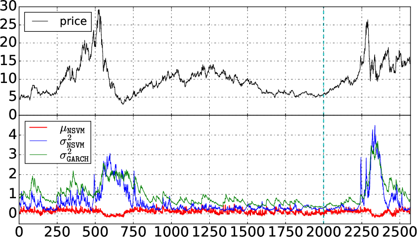
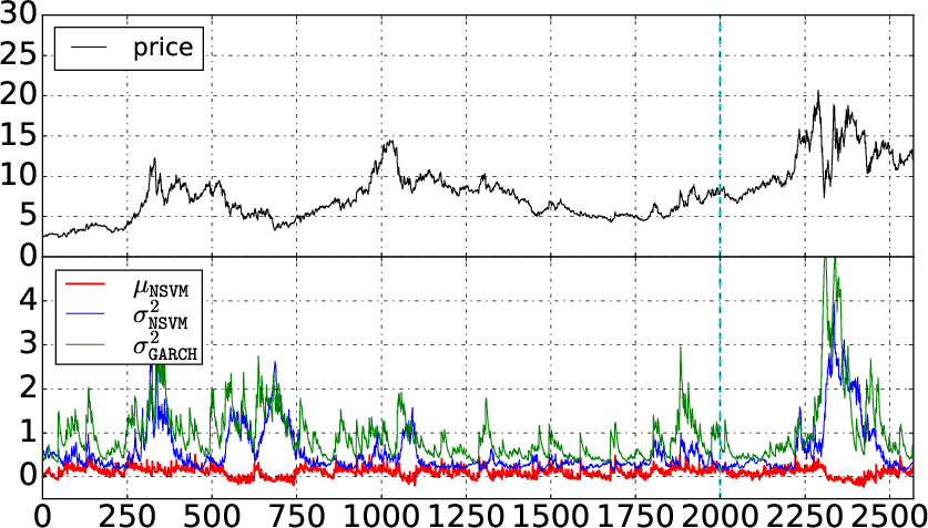
Figure 5: Case studies of volatility forecasting.

Implications and Future Directions

The NSVM represents a significant advancement in volatility modeling by combining the strengths of statistical models and deep learning. The model's flexibility and expressive power allow it to capture complex temporal dependencies and handle multivariate data, overcoming the limitations of traditional approaches. The experimental results demonstrate the NSVM's superior performance in volatility estimation and prediction on real-world financial datasets.

The paper suggests several avenues for future research, including the modeling of time series with non-Gaussian residual distributions, such as heavy-tailed distributions like LogNormal and Student's t-distribution. Further exploration of advanced network architectures and training methods could also improve the model's performance and scalability.